Let’s suppose we wish to minimize a function of parameters, such as the sum of the squares of the residuals. We earlier supposed that the dependency of the residuals to the parameters was linear, and therefore the dependency of the function to the parameters is simply quadratic.
If there is only one parameter, the function will be a simple parabola, if two, a paraboloid. If n parameters, we then should imagine some kind of hyper-paraboloid… We can easily plot this function, with its value on the z-axis, and the parameter vector in the horizontal plane. Of course, we need to be able to imagine that a vector space of dimension n can be represented in a horizontal plane, but us readers of this blog don’t lack imagination, do we? In addition, we know that this paraboloid has a unique minimum, which is very easy to find. So finding our solution should be quite straightforward.
Now, let’s suppose that our vector space is of dimension 6561. For example, the vector space of gravity fields in spherical harmonics up to degree and order 80. That makes a dimension of 81 x 81 = 6561. Let’s also suppose we are too lazy to calculate a minimum on such a big vector space, and that we prefer to calculate the minimum on a subspace of a smaller dimension, let’s say 2601.
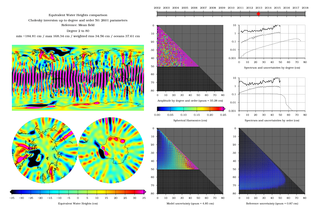
We could take the first subspace that comes to hand, for example the vector space of gravity fields up to degree and order 50, which has the desired dimension. We then could find the minimum in this subspace, and it would provide our gravity solution. This would lead us to the following image:

Finding a solution is quite rewarding. Nonetheless, this image will also inevitably later lead us to reflections and refinements on how to get rid of these annoying stripes all across the picture.
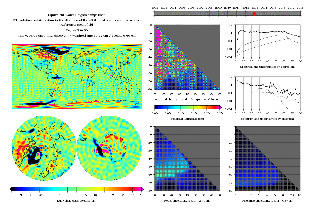
Now we could also try to consider the subspace generated by the 2601 steepest principal axes of the paraboloid. After all, this vector space has the same dimension, so it should lead to comparable results. This method has a very seducing virtue, which is that finding a minimum along the steepest axes is very efficient. You will go down very quickly, while not needing to move too much horizontally. As a bonus, you will also not get too far away from this linearity zone for which the paraboloïd does make some sense. With this attempt, you would find the following gravity solution:

In both cases, we used the same number of parameters : 2601. For a same number of parameters, the difference is quite eloquent. Not only did we get rid of the annoying stripes, but also did we obtain a very nice spatial resolution. Of course, everything is not perfect: there are specific problems that appear, namely at the poles. But with such a remarkable and promising difference, the process definitely deserves some more research and exploration…
On the importance of concentrating efforts in the right direction (the direction of eigenvectors).
(to be continued…)
Stéphane Bourgogne, Saab Abou-Jaoudé and Jean-Michel Lemoine
Géode & Cie and CNES, Toulouse, France
